LyricalSimilarity

Project Title: Kindred Lyrics

Jumshaid Yamin, Andrew Young, William Zheng

Introduction

Background

Music is important. According to the 2017 Music 360 report by Nielsen.com, Americans spent an average of roughly 32 hours per week listening to music. However, not all music is the same – there is a variety of instrumentation, rhythmic styles, tempos, and more abstract things such as mood and lyrical meaning. Depending on how someone feels at the moment, he or she might enjoy a certain type of music. Often what one wants to listen at a certain time depends on the more complex matter of a song’s mood and lyrical content. For example, a song with encouraging lyrics to make someone feel better such as Happy by Pharell Williams. So while it is easy to categorize a song by its BPM – this can be done in a brute force manner – measuring a song’s lyrical content may be a way to provide music listeners with songs that can target their feelings directly.

Motivation

We think that people would like to find songs that match a particular mood or theme. For example, someone might enjoy the theme of a particular song, and he or she may want to find songs with similar lyrical themes.

Problem

Unlike raw, fundamental attributes of a song, such as BPM or volume, lyrical content is complex and difficult to process. When humans understand lyrics, they make full use of their natural language processing abilities, which includes understanding vocabulary, order of words (grammar), and even context. Even then, some songs’ lyrics are sometimes abstract, using metaphors or obtuse, using difficult vocabulary, so not all lyrics are understood by humans. Sometimes, a song’s lyrics are simply nonsensical. Therefore, creating a perfectly program that perfectly understood lyrics would require better understanding than humans, and nonsensical lyrics would need to be dealt with appropriately. The database available to us, Million Song Dataset (MSD) does not provide lyrics in their original form, but in a Bag of Words (BoW) format. This means that instead of giving full sentences, MSD gives us each word in song’s lyrics, and that word’s corresponding frequency. Therefore, it is already impossible to make full use of natural language processing, because we no longer have access to the ordering of words or sentences of the original lyrical text. The project’s problem, therefore, becomes to make full use of the vocabulary to understand the relationship between the lyrics of different songs.

Methods

Data

The lyrics data is already provided to us in the form of an SQL database, where each row represents the frequency of a word in a song. Our goal is to find the similarity between lyrics, but there are no predefined similarities assigned by humans. In other words, there are no labels for our model to learn on. As a consequence, we had to apply unsupervised learning techniques to find the inherent similarities.

Data Processing

Restricting Language

The lyrics database contains songs of many different languages, including Spanish, German, and French. When all languages are present in the dataset, the greatest variance lies in the difference in language. To avoid our model from fixating on such a difference, and therefore miss the more detailed differences between songs of the same language, we decided to restrict the dataset to a single language. We chose English both for convenience and because most of the songs are in English. To filter the data, we used a rule of thumb: if the document does not have at least 3 words among a taylored set of common English words, it is considered another language and is dropped from the dataset. We took some time to pick a good set of words, as our original set included the word “me”, which is common in both English and Spanish.

TF-IDF

The first technique we tried was TF-IDF: term frequency and inverse document frequency. This is where each word of each document is weighted as such:

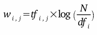
where tf_i,j is the relative frequency of the word i in the document j, and df_i is the frequency of the word i in the entire corpus. Relative frequency means the proportion of frequency of the word in the document and the length of the document. In other words, it’s the normalized frequency of the word. This is used so that larger documents are not overpicked by our algorithm, since they have a larger chance of sharing words with other documents. The IDF aspect of TF-IDF is very helpful because it decreases the importance of common words. For example, two documents should not be considered similar because they both use the word “the” many times. We used sklearn’s TfidfVectorizer class to find the TF-IDF values of our data. TfidfVectorizer expects an array of string sentences as an input, so we transformed each song’s BoW intro an artificial sentence by concatenating the words.

Cosine Similarity & Linear Kernel

After attaining our TF-IDF, we used a technique called cosine similarity to find the similarity between two documents. Cosine similarity is where the angle between two vectors in N-dimensional space represents the similarity between the two vectors. In this case, our vectors are the sparse vectors of the TF-IDF weights of the words in the documents. We used sklearn’s linear_kernel to calculate the similarity between all TF-IDF pairs. Linear kernel operates the same as cosine similarity except it doesn’t normalize the values. However, TfidfVectorizer normalized the values for us, so linear kernel works fine. Stopwords Despite using TF-IDF, which should diminish the weight of common words, we found it necessary to remove stop words. Stop words are words that provide structural information, but nearly no content information. Considering further that our dataset does not include word order, and these words are almost meaningless. Therefore, we tested performance after removal of stopwords. Dimensionality reduction

Dimensionality Reduction

PCA

PCA or Principal Component Analysis is a statistical transformation of possibly correlated features into linearly uncorrelated features called principal components where the first and following principal components contain the greatest share of variance of the dataset. In our case to visualize the data, we attempted PCA with 2 principal components for visualization purposes as well as varying the number of components and using the elbow method to find the optimal number.

TSNE

TSNE or T-distributed Stochastic Neighbor Embedding is a dimensionality reduction algorithm focused for visualization. It is made for transforming high-density (large feature count) data into two or three dimensional space so that it can be easily visualized. This made it well-suited for our needs as we needed to visualize song data in which each feature was word count (where the total numbers of features were over 5000) into a two dimensional space scatter plot.

Clustering Algorithms

K-MEANS

K-means is a clustering algorithm where n observations are partitioned into k clusters where each observation belongs to the cluster with the nearest mean. K-means is best for when visual clusters exist as it disregards density. We ran K-means with a varying number of clusters with a PCA with 2 components as well as a varying number of components as well as TSNE with 2 dimensions.

DBSCAN

DBSCAN or Density-based spatial clustering of applications with noise is a clustering algorithm that groups observations together that are closely packed leaving outlier not in any cluster. We ran DBSCAN with varying epsilons with TSNE with 2 dimensions and PCA with two components.

Clustering Evaluation Algorithms

We used silhouette score to evaluate our clusters. We iterated through many values of epsilon for DBSCAN in order to find the best value. Silhouette value is a measure of how similar an object is to its own cluster (cohesion) compared to other clusters (separation). The silhouette ranges from −1 to +1, where a high value indicates that the object is well matched to its own cluster and poorly matched to neighboring clusters. If most objects have a high value, then the clustering configuration is appropriate. If many points have a low or negative value, then the clustering configuration may have too many or too few clusters.

Results

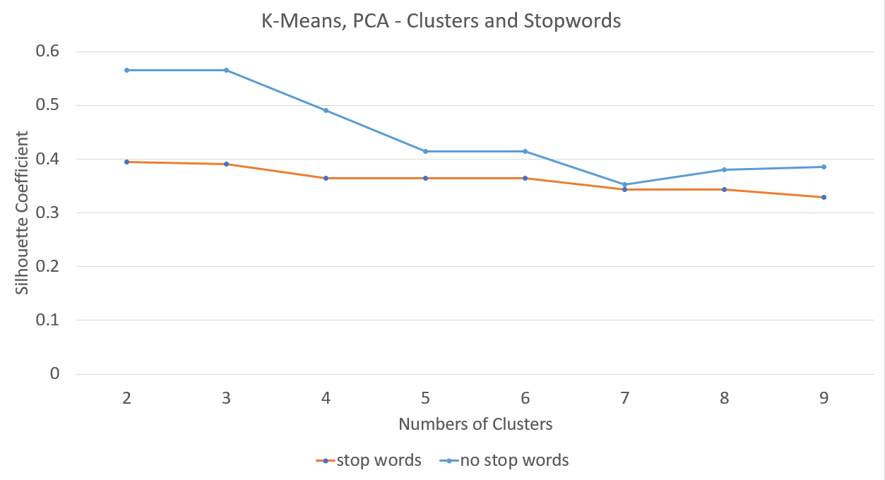
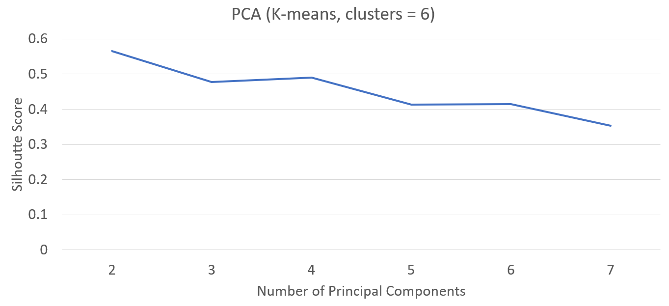
K-means with PCA Varying Number of Clusters, Stop Words and No Stop Words

K means with TSNE and Varying clusters

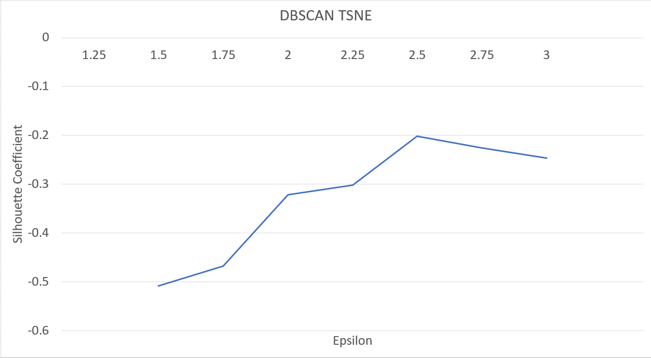
DBSCAN with PCA and Varying Epsilon

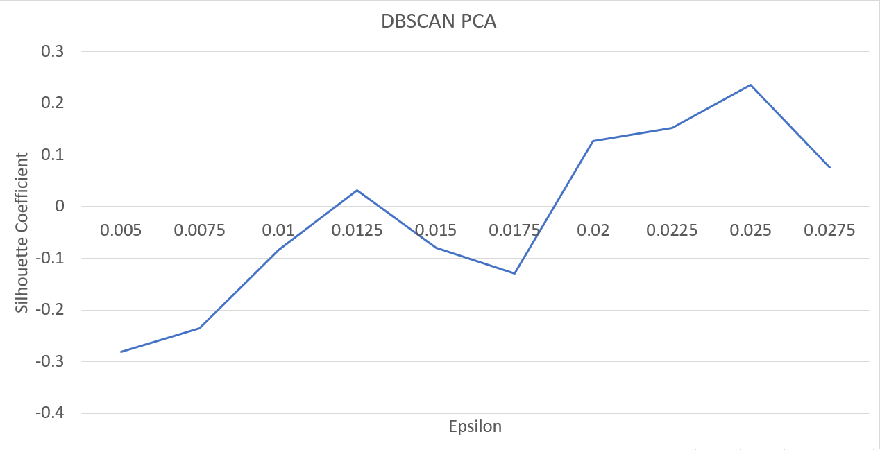
DBSCAN with TSNE and Varying Epsilon

Finding Optimal Number of Components using Silhouette Score

Clusterings

K-Means did not provide very good clusters:

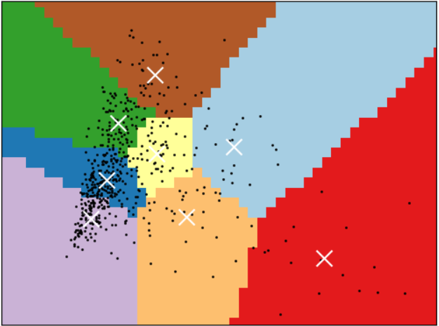
The black points are the data points, and the white Xs are the cluster centroids. DBSCAN gave better results.

We found that despite our use of TF-IDF, removing stopwords beforehand increased the accuracy of our clusters.

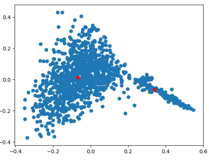
^Data before removing stopwords

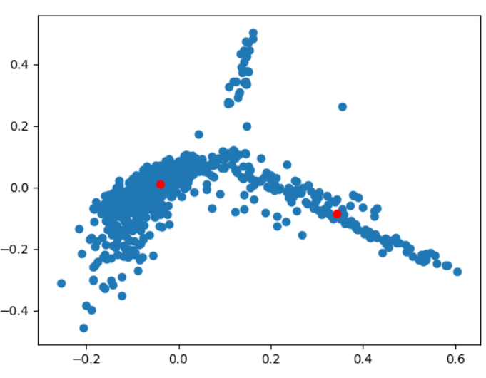
^Data after removing stopwords

We found that removing non-English lyrics improved performance significantly. The clusters become sharper and better defined. Here is the difference between before and after we restricted language:

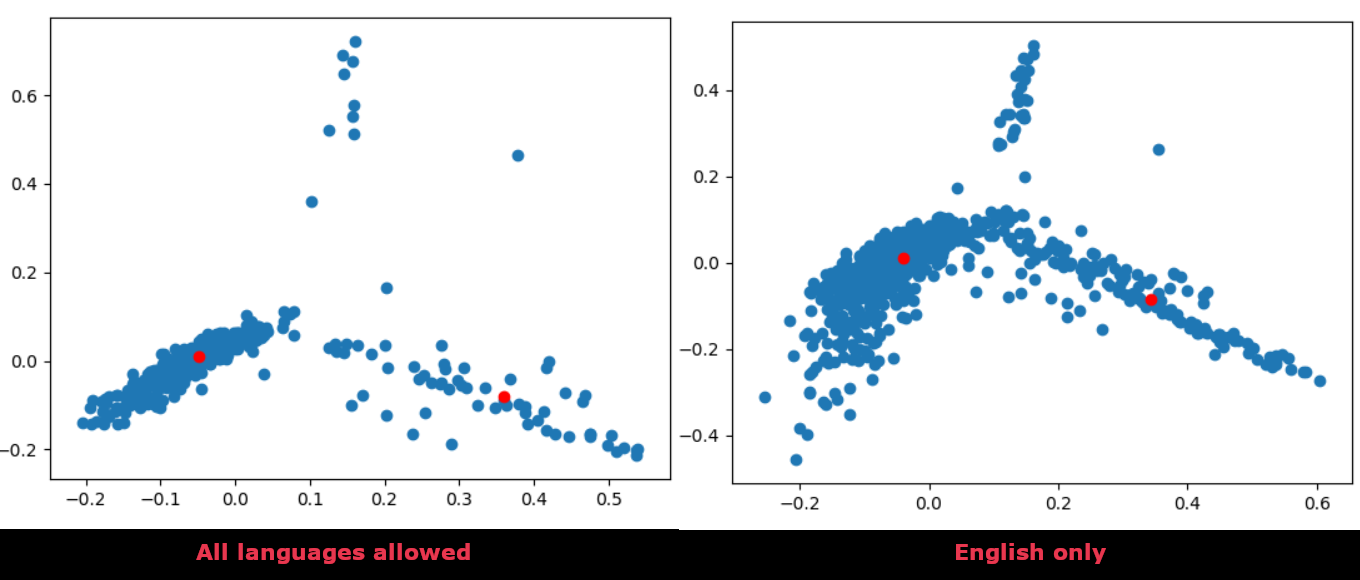
The data gets closer together, since all the data points are now connected through a common freature, their language. The remaining islands may be languages that slipped through our rule-of-thumb language detector, though.

We achieved our best results with the following configuration: graph_maker(‘tsne’, ‘dbscan’, no_stopwords=True, components=2, eps=1.9, cluster_num=8) and min_pts = 3

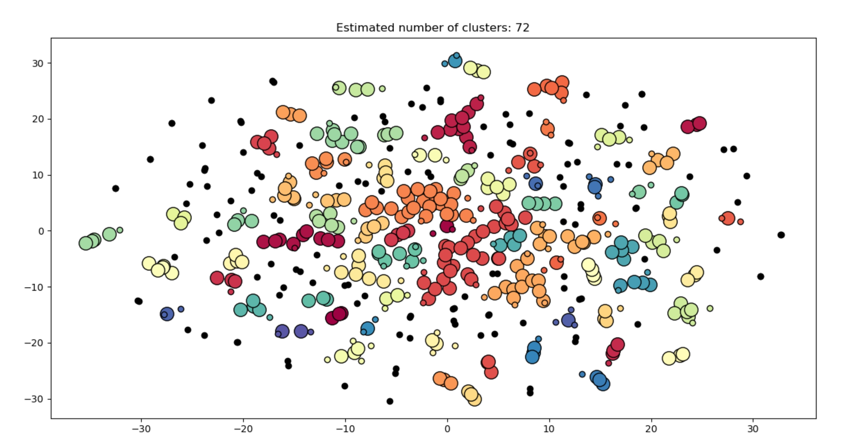
Which means that we restricted the language to English, removed stopwords, fed our data into TF-IDF, performed TSNE dimensionality reduction, and used DBSCAN to cluster the data in the new feature space. The clusters were pretty good – we found a cluster of songs whose vocabulary consists of words like “love” and “dream”. We also found a cluster of lyrics filled with curse words.

Discussion

PCA vs. TSNE

In general, we found that dimensionality reduction using TSNE visually and lyrically outperformed reduction using Principal Component Analysis. The songs in each cluster made from TSNE often appeared more lyrically similar than those from PCA. This is perhaps because the purpose of TSNE was to prioritize the reduction to two or three dimensional space (from a high-dimension space) so that the data could be visually displayed in a scatter plot such as ours. However, based on Silhouette values, PCA generally fared better as each song was more closely matched to its cluster and not others.

DBSCAN vs. K-Means

K-Means finds clusters by finding linear boundary lines between the data. So K-Means assumes that the optimal clusters are linearly separable. DBSCAN makes no such assumption and is able to find more complex patterns. Furthermore, DBSCAN is robust to noise, of which our data has a lot. This is likely due to the spread of the data as there existed pockets of high density points while the data itself was not clearly defined into clusters. These conditions make DBSCAN the better clustering algorithm. It therefore makes sense that DBSCAN performed better than K-Means.

Silhouette Coefficient

We found empirically that the silhouette coefficient was not a good evaluator of our clusters. We found the epsilon value that maximized the silhouette coefficient, but the associated clusters were few and noisy. We are not sure why the silhouette coefficient gave higher scores for clusters that were empirically bad. Perhaps it is ill-suited for our data, or for our representation of our data.

Future Work

We managed to get decent clusters with TF-IDF, TSNE, and DBSCAN, but we could not achieve sensible clusters using meaning-based word embeddings. If we were to continue this project, we would want to get Word2Vec to work, so that we could find lyrics with similar-meaning words. Furthermore, we would want to clean our data more thoroughly, using more rigorous checks for language (rather than our rule of thumb). Discarding bilingual songs is another consideration. Continuing the project, we would also try other cluster evaluation methods, such as the Davies–Bouldin index, so we could find better epsilon values for DBSCAN.

References

Dataset: http://millionsongdataset.com/musixmatch/

1. Gomaa, W. H. (2013). A Survey of Text Similarity Approaches. International Journal of Computer Applications, Volume 68, No. 13.
2. Corley, C., Mihalcea, R., Strapparava, C. (2006). AAAI’06 Proceedings of the 21st national conference on Artificial intelligence – Volume 1.
3. Sieg, A. (2018). Text Similarities : Estimate the degree of similarity between two texts. Medium. https://medium.com/@adriensieg/text-similarities-da019229c894.
4. Heuer H. (2016). Text comparison using word vector representations and dimensionality reduction. CoRR, abs/1607.00534.